Nonlinear regression is used to see whether one continuous variable is correlated with another continuous variable, but in a nonlinear way, i.e. when a set of x vs. y data you plan to collect do not form a straight line, but do fall on a curve that can be modelled in some sensible way by a known equation, e.g.

Some important general considerations for fitting models of this sort include:

• The model must make physical sense. R (and Excel) can happily stick polynomial curves (e.g. a cubic like y=ax³+bx²+cx+d) through a data set, but fitting random equations through data is a pointless exercise, as the values of a, b, c and d are meaningless and do not relate to some useful quantity that characterises the behaviour of the data. If you want to fit a curve to a data set, it has to be a curve (and therefore an equation) you’ve chosen because it estimates something meaningful (e.g. the Michaelis constant, K_M).
• There must be enough data points. In general, you cannot fit a useful model of n parameters to a data set smaller than n+1 in size. In linear regression, you cannot fit a slope and an intercept (2 parameters) to just one datum, as there are an infinite number of lines that pass through a single point and no way to choose between them. You shouldn’t fit a 2 parameter model to 2 data points as this doesn’t buy you anything: your model is at least as complex as a simple list of the two data values. The Michaelis-Menten model has two parameters, so you need at least three concentrations of S, and preferably twice this. As ever, collect the data needed for the analysis you plan to do; don’t just launch into collecting the data and then wonder how you will analyse it, because often the answer will be “with great difficulty” or “not at all”.
• The data set should aim to cover the interesting span of the response, even if you don’t really know what that span is. A linear series of concentrations of S is likely to miss the interesting bit of an enzyme kinetic curve (around K_M) unless you have done some preliminary experiments. Those preliminary experiments will probably need to use a logarithmic series of concentrations, as this is much more likely to span the interesting bit. This is particularly important in dose/response experiments: use a concentrations series like 2, 4, 8, 16…mM, or 10, 100, 1000, 10000…µM, rather than 2, 4, 6, 8, 10…mM or 10, 20, 30, 40…µM; but bear in mind the saturated solubility (and your own safety!) when choosing whether to use a base-2, a base-10, or base-whatever series.

The data in enzyme_kinetics.csv gives the velocity, v, of the enzyme acid phosphatase (µmol min⁻¹) at different concentrations of a substrate called nitrophenolphosphate, [S] (mM). The data can be modelled using the Michaelis-Menten equation given at the top of this post, and nonlinear regression can be used to estimate K_M and v_max without having to resort to the Lineweaver-Burk linearisation.

In R, nonlinear regression is implemented by the function nls(). It requires three parameters. These are:

• The equation you’re trying to fit
• The data-frame to which it’s trying to fit the model
• A vector of starting estimates for the parameters it’s trying to estimate

Fitting a linear model (like linear regression or ANOVA) is an analytical method. It will always yield a globally optimal solution, i.e. a ‘perfect’ line of best fit, because under the hood, all that linear regression is doing is finding the minimum on a curve of residuals vs. slope, which is a matter of elementary calculus. However, fitting a nonlinear model is a numerical method. Under the hood, R uses an iterative algorithm rather than a simple equation, and as a result, it is not guaranteed to find the optimal curve of best fit. It may instead get “jammed” on a local optimum. The better the starting estimates you can give to nls(), the less likely it is to get jammed, or – indeed – to charge off to infinity and not fit anything at all.

For the equation at the start of this post, the starting estimates are easy to estimate from the plot:

enzyme.kinetics<-read.csv( "H:/R/enzyme_kinetics.csv" )
plot(
    v ~ S,
    data = enzyme.kinetics,
    xlab = "[S] / mM",
    ylab = expression(v/"µmol " * min^-1),
    main = "Acid phosphatase saturation kinetics"
)

The horizontal asymptote is about v=9 or so, and therefore K_M (value of [NPP] giving v_max/2) is about 2.

The syntax for nls() on this data set is:

enzyme.model<-nls(
    v ~ vmax * S /( KM + S ),
    data  = enzyme.kinetics,
    start = c( vmax=9, KM=2 )
)

The parameters in the equation you are fitting using the usual ~ tilde syntax can be called whatever you like as long as they meet the usual variable naming conventions for R. The model can be summarised in the usual way:

summary( enzyme.model )

Formula: v ~ vmax * S/(KM + S)
Parameters:
     Estimate Std. Error t value Pr(>|t|)    
vmax 11.85339    0.05618  211.00 7.65e-13 ***
KM    3.34476    0.03860   86.66 1.59e-10 ***
---
Signif. codes: 
0 '***' 0.001 '**' 0.01 '*' 0.05 '.' 0.1 ' ' 1 

Residual standard error: 0.02281 on 6 degrees of freedom
Number of iterations to convergence: 4 
Achieved convergence tolerance: 6.044e-07

The curve-fitting has worked (it has converged after 4 iterations, rather than going into an infinite loop), the estimates of K_M and v_max are not far off what we made them by eye, and both are significantly different from zero.

If instead you get something like this:

Error in nls( y ~ equation.blah.blah.blah, ): singular gradient

this means the curve-fitting algorithm has choked and charged off to infinity. You may be able to rescue it by trying nls(…) again, but with different starting estimates. However, there are some cases where the equation simply will not fit (e.g. if the data are nothing like the model you’re trying to fit!) and some pathological cases where the algorithm can’t settle on an estimate. Larger data sets are less likely to have these problems, but sometimes there’s not much you can do aside from trying to fit a simpler equation, or estimating some rough-and-ready parameters by eye.

If you do get a model, you can use it to predict the y values for the x values you have, and use that to add a curve of best fit to your data:

# Create 100 evenly spaced S values in a one-column data frame headed 'S'
predicted.values <- data.frame(
    S = seq( 
       from       = min( enzyme.kinetics$S ),
       to         = max( enzyme.kinetics$S ),
       length.out = 100
    )
)

# Use the fitted model to predict the corresponding v values, and assign them
# to a second column labelled 'v' in the data frame
predicted.values$v <- predict( enzyme.model, newdata=predicted.values )

# Add these 100 x,y data points to the graph, joined up by 99 line-segments
# This will look like a curve at the resolution of the graph
lines( v ~ S, data=predicted.values )

If you need to extract a value from the model, you need coef():

vmax.estimate <- coef( enzyme.model )[1]
KM.estimate   <- coef( enzyme.model )[2]

This returns the first and second coefficients out of the model, in the order listed in the summary().

Exercises

Try fitting non-linear regressions to the data sets below

1. Estimate the doubling time from the bacterial data set in bacterial_growth.csv. N is the optical density of bacterial cells at time t; N₀ is the OD at time 0 (you’ll need to estimate N₀ too: it’s ‘obviously’ 0.032, but this might have a larger experimental error than the rest of the data set). t is the time (min); and t_d is the doubling time (min).

2. The response of a bacterium’s growth rate constant μ to an increasing concentration of a toxin, [X], is often well-modelled by a sigmoidal equation of the form below, with a response that depends on the log of the toxin concentration. The file dose_response.csv contains data on the response of the growth constant μ (“mu” in the file, hr^‑1) in Enterobacter sp. to the concentration of ammonium ions, [NH₄⁺] (“C” in the file, µM). The graph below shows this data plotted with a nonlinear regression curve. Reproduce it, including the superscripts, Greek letters, italics, etc., in the axis titles; and the smooth curve predicted from the fitted model.

• μ is the exponential phase growth constant (hr⁻¹) at any given concentration of X.
• μ_max is the maximum value that μ takes, i.e. the value of μ when the concentration of toxin, [X], is zero. The starting estimate should be is whatever the curve seems to be flattening to on the left.
• IC₅₀ is the 50% inhibitory concentration, i.e. the concentration of X needed to reduce μ from μ_max to ½μ_max. The starting estimate of ln IC₅₀ should be the natural log of the value of [X] that gives you half the maximum growth rate.
• s is the shape parameter: if s is small the curve drops off sharply like a cliff-edge; if s is large, the curve slopes more gently. If s is negative, the curve is Z-shaped; if s is positive, the curve is S-shaped. It starting estimate should be (ln IC₂₅ − ln IC₇₅) / 2, where IC₂₅ is the concentration needed to reduce μ by 25%, and IC₇₅ is the concentration needed to reduce μ by 75%. If you wish to prove this to yourself, pretend that e=3 rather than 2.718… and work out what [X] has to be to give you this value.
• Note the x-variable in the equation and on the plot is the natural logarithm of [X], so you’ll need to use log(C) in your calls to plot() and nls().

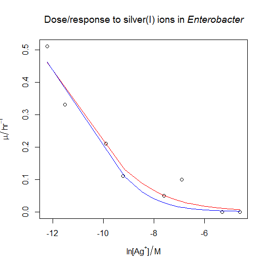
3. The bacterium from the previous question is also sensitive to silver(I) ions. The file dose_response_tricky.csv contains μ values (“mu” in the file, hr^‑1) in Enterobacter sp. at various concentrations of the silver(I) ion, [Ag⁺] (“C” in the file, M). Unfortunately, the data does not span all of the interesting part of the response. Try fitting the three-parameter sigmoidal from the previous question. What happens? Can you justify and fit a simpler model?
4. On islands, the number of species tends to increase with the area of the island, but typically as some power-law, rather than proportionally. This is usually modelled with the simple formula shown below, where S is the number of species, A is the area of the island, C is a scaling factor that depends on the choice of area unit, and z is the power-law parameter of interest. Use nonlinear regression to fit this model to the data in carribean_herps.csv (based on Darlington, 1957), which gives the total number of reptile+amphibian (‘herps’) species on seven caribbean islands of varying sizes. You will need to estimate starting parameters for C and z. The traditional way to calculate these parameters is to transform the equation to a linear form using logarithms, and then fit a linear model. You can use this technique to estimate the starting parameters.

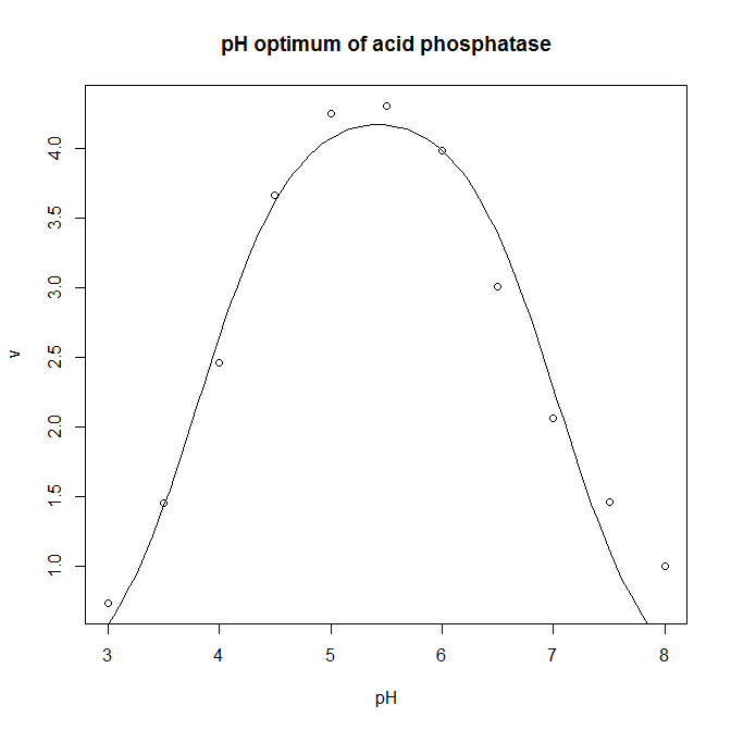
5. The pH optimum of an enzyme can be modelled by the Michaelis model shown below, where v is the velocity of the enzyme, v₀ is the velocity at the pH optimum, H is the concentration of hydrogen ions (H = [H⁺]= 10^−pH), and K_a and K_b are two apparent dissociation constants for residues in the active site of the enzyme. ph_optimum.csv gives velocities at various pH values for the enzyme acid phosphatase. v₀ is easily eye-balled from the graph. K_a and K_b can also be easily estimated: the line v= v₀/2 will intersect the pH dependence curve at two points, one to the left of the optimum, and one to the right: if you drop vertical lines down to the pH axis from each of these two intersections, the left-hand this vertical line cuts the pH axis at the pK_a (which is −log₁₀(K_a), and the right-hand oen cuts at the pK_b (which is −log₁₀(K_b). Plot the pH dependence curve, and use nonlinear regression to estimate the parameters, and from that the pH optimum, pH_opt = −log₁₀(√K_aK_b).

Answers

1. The doubling time t_d is around 25 min.

bacterial.growth<-read.csv( "H:/R/bacterial_growth.csv" )
plot(
    N    ~ t,
    data = bacterial.growth,
    xlab = "N",
    ylab = "t / min",
    main = "Bacteria grow exponentially"
)

head( bacterial.growth )

   t    N
1  0 0.032
2 10 0.046
…

We estimate the parameters from the plot: N₀ is obviously 0.032 from the data above; and the plot (below) shows it takes about 20 min for N to increase from 0.1 to 0.2, so t_d is about 20 min.

bacterial.model<-nls(
    N     ~ N0 * exp( (log(2) / td ) * t),
    data  = bacterial.growth,
    start = c( N0 = 0.032, td = 20 )
)
summary( bacterial.model )

Formula: N ~ N0 * exp((log(2) / td) * t)
Parameters:
    Estimate Std. Error t value Pr(>|t|)    
N0 3.541e-02  6.898e-04   51.34 2.30e-11 ***
td 2.541e+01  2.312e-01  109.91 5.25e-14 ***
---
Signif. codes: 
0 '***' 0.001 '**' 0.01 '*' 0.05 '.' 0.1 ' ' 1 
Residual standard error: 0.002658 on 8 degrees of freedom
Number of iterations to convergence: 5 
Achieved convergence tolerance: 1.052e-06

This bit adds the curve to the plot below.

predicted.values <- data.frame( 
    t = seq( 
       from       = min( bacterial.growth$t ),
       to         = max( bacterial.growth$t ),
       length.out = 100
    )
)
predicted.values$N <- predict( bacterial.model, newdata = predicted.values )
lines( N ~ t, data = predicted.values )

2. Dose/response model and graph

dose.response<-read.csv( "H:/R/dose_response.csv" )
plot(
    mu   ~ log(C),
    data = dose.response,
    xlab = expression("ln" * "[" * NH[4]^"+" * "]"
/ µM),
    ylab = expression(mu/hr^-1),
    main = expression("Sigmoidal dose/response to ammonium ions in " *
italic("Enterobacter"))
)

The plot indicates that the starting parameters should be

• μ_max ≈ 0.7
• ln IC₅₀ ≈ ln(3), because IC₅₀ is the value of [X] corresponding to μ_max/2 ≈ 0.35, and this is about 3. You can see this by inspecting the raw data (the mid μ value is caused by an [X] somewhere between 2 and 4), or by looking at the plot (where the mid μ value corresponds to a ln([X]) of about 1). We’ll call ln(IC₅₀) logofIC50 in the formula to nls() below so it’s clear this is a parameter we’re estimating, not a function we’re calling.
• s ≈ − 0.6, because s ≈ (ln IC₂₅− ln IC₇₅) / 2 ≈ (ln(1.5) − ln(6)) / 2 ≈ (0.4 − 1.8) / 2. IC₂₅ is the concentration needed to reduce μ by 25% (μ = 0.525, corresponding to about 1.5 µM), and IC₇₅ is the concentration needed to reduce μ by 75% (μ = 0.175, corresponding to about 6 µM).

dose.model <- nls(
    mu    ~ mumax / ( 1 + exp( -( log(C) - logofIC50 ) / s ) ),
    data  = dose.response,
    start = c( mumax=0.7, logofIC50=log(3), s=-0.7 )
)
summary( dose.model )

Formula: mu ~ mumax/(1 + exp(-(log(C) - logofIC50)/s))
Parameters:
          Estimate Std. Error t value Pr(>|t|)    
mumax     0.695369   0.006123  113.58 1.00e-09 ***
logofIC50 1.088926   0.023982   45.41 9.78e-08 ***
s        -0.509478   0.020415  -24.96 1.93e-06 ***
---
Signif. codes: 
0 '***' 0.001 '**' 0.01 '*' 0.05 '.' 0.1 ' ' 1 
Residual standard error: 0.00949 on 5 degrees of freedom
Number of iterations to convergence: 5 
Achieved convergence tolerance: 6.394e-06
Achieved convergence tolerance: 5.337e-06

This lists the estimates of μ_max, ln(IC₅₀) and s, plus the standard error of these estimates and their p values. Note that they’re all pretty close to what we guessed in the first place, so we can be fairly sure they’re good estimates. To get the actual value of IC₅₀ from the model:

exp( coef(dose.model)[2] )

This gives 2.97 µM, which corresponds well with our initial guess.

To add the curve, we do the same as before:

predicted.values <- data.frame( 
    C = seq( 
       from       = min( dose.response$C ),
       to         = max( dose.response$C ),
       length.out = 100
    )
)
predicted.values$mu <- predict( dose.model, newdata = predicted.values )
lines( mu ~ log(C), data=predicted.values )

Note that in the real world, you might be hard-pressed to fit a 3-parameter model to a data set of just 8 points, because it is unlikely that they would fall so neatly, and with such a convenient range from zero effect to complete inhibition. In the real world, there’s a very good chance that the nonlinear regression would fail, puking up something like:

Singular gradient

Under these circumstances, you can simplify the model you are trying to fit, e.g. by removing the s parameter (setting it equal to minus 1), which simplifies the equation you are trying to fit to:

and requires this modification to the nls():

dose.model <- nls(
    mu    ~ mumax / ( 1 + exp( log(C) - logofIC50 ) ),
    data  = dose.response,
    start = c( mumax=0.7, logofIC50=log(3) )
)

3. Following on from the previous answer, when we try to fit the silver dose/response, the nonlinear regression fails, even when fed reasonable starting estimates. The solution is to try fitting a simpler model with only two parameters rather than three. We can see what happens if we pass the trace=TRUE argument  to nls(): we can see that the estimates diverge as R tries to fit the curve, rather than converging. One option is to fix mumax at the value obtained from the previous answer. This could be justified if the conditions in the ammonium and the silver(I) growth flasks were otherwise identical. The other option is to fix the value of s at −1 , which has the effect of simplifying the equation as described in the answer above. In both cases, the nonlinear regression now works, and gives similar estimates of IC₅₀: I’d probably choose the second option, but really it would be better overall to collect more data at the low concentration end of the curve if time and materials permitted.

dose.response<-read.csv( "H:/R/dose_response_tricky.csv" )
plot(
    mu   ~ log(C),
    data = dose.response,
    xlab = expression("ln" * "[" * Ag^"+" * "]" / M),
    ylab = expression(mu/hr^-1),
    main = expression("Dose/response to silver(I) ions in " * italic("Enterobacter"))
)

# Three parameter model

dose.model <- nls(
    mu    ~ mumax / ( 1 + exp( -( log(C) - logofIC50 ) / s ) ),
    data  = dose.response,
    start = c( mumax=0.7, logofIC50=log(1e-5), s=-2 ),
    trace=TRUE
)

The output shows divergence (the numbers in the columns are the values of mumax, logofIC50 and s respectively:

0.01784401 :    0.70000 -11.51293  -2.00000
0.01628421 :    0.8985258 -12.5957842  -2.1549230
0.01542858 :    1.061574 -13.223248  -2.218839
0.01507904 :    1.278977 -13.899840  -2.275899
0.01465342 :    1.429477 -14.271384  -2.301364
0.01435196 :    1.610375 -14.662795  -2.325330
0.01419041 :    1.831461 -15.078767  -2.347909
...
Error in nls(mu ~ mumax/(1 + exp(-(log(C) - logofIC50)/s)), data = dose.response,  : 
  number of iterations exceeded maximum of 50

Option one: fix the value of mumax to the value from the previous answer. This gives us a natural log of IC₅₀ of −11.2386.

# Fix mumax

dose.model.fixed.mumax <- nls(
    mu    ~ 0.695 / ( 1 + exp( -( log(C) - logofIC50 ) / s ) ),
    data  = dose.response,
    start = c( logofIC50=log(1e-5), s=-2 )
)

predicted.values.fixed.mumax <- data.frame( 
    C = seq( 
       from       = min( dose.response$C ),
       to         = max( dose.response$C ),
       length.out = 100
    )
)

predicted.values.fixed.mumax$mu <- predict( dose.model.fixed.mumax, 
newdata = predicted.values.fixed.mumax )

lines( mu ~ log(C), data=predicted.values.fixed.mumax, col='red' )

Option two: fix the value of s to −1. This gives us a natural log of IC₅₀ of −10.55757.

# Fix shape

dose.model.fixed.s <- nls(
    mu    ~ mumax / ( 1 + exp( log(C) - logofIC50 ) ),
    data  = dose.response,
    start = c( mumax=0.7, logofIC50=log(1e-5) )
)

summary( dose.model.fixed.s )

predicted.values.fixed.s <- data.frame( 
    C = seq( 
       from       = min( dose.response$C ),
       to         = max( dose.response$C ),
       length.out = 100
    )
)

predicted.values.fixed.s$mu <- predict( dose.model.fixed.s, 
newdata = predicted.values.fixed.s )

lines( mu ~ log(C), data=predicted.values.fixed.s, col='blue' )

4. We use linear regression on the log values to estimate C and z, then we use these values as the starting parameters for the nonlinear regression.

caribbean.herps<-read.csv( "H:/R/caribbean_herps.csv" )

plot(
    Species ~ Area,
    data = caribbean.herps,
    xlab = expression("Area / " * km^2),
    ylab = "Number of species of amphibians and reptiles",
    main = "Larger islands have more species, but not proportionally so"
)

# Species/area relationship is a power law, so reasonable starting parameters
# can be taken from a log/log plot: if S = CA^z, then log S = log C + z log A

loglog.model<-lm(
    log(Species) ~ log(Area),
    data = caribbean.herps,
)

# Extract the slope and intercept (named vectors) from the linear model on 
# the log/log values, extract the numerical values of these parameters from
# the named vectors, and back-transform the intercept (log C) to get C itself

C.estimate<-exp( as.numeric( coef(loglog.model)[1] ) )
z.estimate<-as.numeric( coef(loglog.model)[2] )

nls.model <- nls(
    Species ~ C*Area^z,
    data    = caribbean.herps,
    start   = c( C=C.estimate, z=z.estimate )
)

summary( nls.model )

predicted.values <- data.frame( 
    Area = seq( 
       from       = min( caribbean.herps$Area ),
       to         = max( caribbean.herps$Area ),
       length.out = 100
    )
)

predicted.values$Species <- predict( nls.model, newdata = predicted.values )

lines( Species ~ Area, data=predicted.values )

The linear model on the log transformed variables gives estimates of C = 2.6 and z=0.30; the nonlinear model on the raw data then gives estimates of C = 1.6 and z=0.35. You’ll note the estimates are rather different.

5. The optimum is 5.4.

ph.optimum<-read.csv( "H:/R/ph_optimum.csv" )

plot(
	v   ~ pH,
	data = ph.optimum,
	xlab = "pH",
	ylab = "v",
	main = "pH optimum of acid phosphatase"
)

ph.model <- nls(
	v     ~ v0 / ( 1 + (10^-pH)/Ka + Kb/(10^-pH) ),
	data  = ph.optimum,
	start = c( v0=7, Ka=10^-4, Kb=10^-7 )
)
summary( ph.model )

predicted.values <- data.frame( 
	pH = seq( 
		from       = min( ph.optimum$pH ),
		to         = max( ph.optimum$pH ),
		length.out = 100
	)
)
predicted.values$v <- predict( ph.model, newdata=predicted.values )
lines( v ~ pH, data=predicted.values )

# This calculates the optimum pH:

-log10(sqrt(coef(ph.model)[2]*coef(ph.model)[3]))